Deep Recurrent Neural Networks (in Java)

https://github.com/evolvingstuff/RecurrentJava

My favorite machine learning papers from the last 6 months

Compete to Compute
Inferring Algorithmic Patterns with Stack-Augmented Recurrent Nets
Invariant backpropagation: how to train a transformation-invariant neural network
Memory Networks
Towards AI-Complete Question Answering: A Set of Prerequisite Toy Tasks
DRAW: A Recurrent Neural Network For Image Generation
Show, Attend and Tell: Neural Image Caption Generation with Visual Attention
Delving Deep into Rectifiers: Surpassing Human-Level Performance on ImageNet Classification
A New Framework to Probe and Learn Neural Networks
Text Understanding from Scratch
Do Deep Nets Really Need to be Deep?
Effective Use of Word Order for Text Categorization with Convolutional Neural Networks
Why does Deep Learning work? - A perspective from Group Theory
FitNets: Hints for Thin Deep Nets
Exploring Invariances in Deep Convolutional Neural Networks Using Synthetic Images
Deep Fried Convnets
Deep Speech: Scaling up end-to-end speech recognition
Recurrent Models of Visual Attention
Teaching Deep Convolutional Neural Networks to Play Go
Deep Neural Networks are Easily Fooled: High Confidence Predictions for Unrecognizable Images
An exact mapping between the Variational Renormalization Group and Deep Learning
Advances in Optimizing Recurrent Networks
Very Deep Convolutional Networks for Large-Scale Visual Recognition
k-Sparse Autoencoders
A Clockwork RNN
Random feedback weights support learning in deep neural networks
Learning to Execute
Neural Turing Machines

Visualizing Individual Neuron Activations in Deep Neural Networks

Each of the pictures above corresponds to the activations of single neurons chosen from within the hidden layers of a deep neural network trained to generate and image of the Mona Lisa (a task which I've previously described here and here.)

The global inputs to the neural network consist of 2-dimensional tuples of (x, y) coordinates, and this arrangement allows the behavior of single neurons to be visualized completely. Each pixel location corresponds to a different (x, y) input, and the pixel intensity at that location represents the scalar activation of the neuron when the neural network as a whole is exposed to that particular coordinate-pair.

In order to generate each of the images, which when full size are 429-by-300 pixels, the neural network must be run 128,700 times.

Here is the end result:

Learning to Generate Mona Lisa, Animated

This is a follow-up to my previous post. It shows the learning process over the course of 500 epochs. The neural network being used has 4 hidden layers of 300 rectified linear units.

EDIT: I just posted this to reddit, and as pointed out by quotemycode, it wasn't very clear what is going on, so I've added some clarification:

The point of this is not to improve on the original image. Of course, that is a nice goal, but that is not at all what I'm doing here. The point of this is to demonstrate the necessity of using deep, as opposed to shallow, neural networks to generate reasonably good results on this task. The reason I did that was because, while experimenting with a standard benchmark for deep NNs, MNIST (digit recognition), I found it could be solved to almost state-of-the-art levels with a very large single hidden layer. The other standard benchmark tasks are much larger scale, and require extensive use of GPUs to get good results. I, however, do not have access to this level of hardware. The advantage of something like this is that I can get feedback in a matter of minutes using a relatively low-end computer. For example, MNIST is 784 dimensions of input times 60,000 training examples. The image I used here is 300x429. This means that I can run through an epoch of training about 182 times faster than MNIST. This fast feedback loop is really useful when experimenting with different deep architectures. So that is why I'm doing this; it isn't about generating better images, it's about having a faster way to experiment with deep architectures. And it happens to generate some neat looking animations in the process, which is why I posted it.

EDIT 2: Just added source code for this on GitHub: https://github.com/evolvingstuff/MonaLisa

Generating Mona Lisa Pixel By Pixel

I've been experimenting with MNIST for awhile now, and have recently come to the conclusion that it is not a very good problem for highlighting the strengths of deep neural networks. I was able to get near state-of-the-art results (for neural nets; not RBMs), using just a single (albeit large) hidden layer of 6000 rectified linear neurons.

Inspired by a blog post I saw some time ago about about evolving an image of the Mona Lisa, I had an idea for a task that might better highlight the benefits of deep neural networks.

The idea is to use supervised regression to learn a mapping between pixel locations and RGB colors, with the goal of generating an image on pixel at a time. This means that if the dimensions of the target image are X-by-Y, then it is necessary to run the network XY times. If the image is 100-by-100, there will be 10,000 training examples.

All of the locations and RGB values are first normalized to fall into the range [0, 1].

So, as a concrete example, if the pixel in the very middle of an image is beige, then the training example associated with that pixel could look like:

(0.5, 0.5) → (0.96, 0.96, 0.86)

Again, the two values on the left hand side are representative of location, and the three values on the right hand side represent red, green, and blue, respectively.

I've begun doing some preliminary testing of this idea. I'm training neural networks to generate the Mona Lisa, pixel by pixel.

The first picture (above) is the result of training a neural network with a similar architecture to the one I used successfully on the MNIST task. It only uses a single hidden layer.

Now, what happens if we instead use three hidden layers?

The result of using multiple hidden layers is quite perceptibly better.

One drawback is that there is no straightforward way to measure anything like generalization (there are no test or validation sets.) I suppose it might be possible to hide certain small parts of the picture during training to see how well the neural network can fill in the gaps, but this idea seems fraught with difficulties.

However, I'm not overly concerned. Just learning to generate the picture appears to be a very difficult learning challenge, one that already seems to clearly highlight the limitations of shallow neural architectures. So although this task lacks some of the characteristics of those normally found in machine learning, I think there is still much to be gained from further exploration.

EDIT: Just added source code for this on GitHub: https://github.com/evolvingstuff/MonaLisa

MNIST Features

These features are not very pretty, but oddly enough work very well on MNIST.

Learning MNIST with shallow neural networks

EDIT: Source code for this experiment: https://github.com/evolvingstuff/MNIST

I've recently been experimenting with the MNIST task using shallow (only a single hidden layer) neural networks. Interestingly enough, when borrowing some of techniques used in deep neural nets, such as rectified linear neurons, and using a large number of hidden units (6000 in this case), the results are fairly good.  It gets less than 1.2% test error after about 30 passes through the training set.

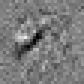
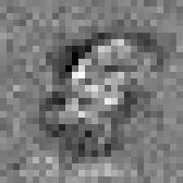
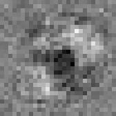
Here are some visual examples of the strength of the link weights connecting the 28-by-28 pixel inputs to the hidden neurons:

SimpleLSTM

A new recurrent neural network architecture I recently came up with inspired by Long Short Term Memory, but simpler:

https://github.com/evolvingstuff/SimpleLSTM

Long Short Term Memory (in Java)

https://github.com/evolvingstuff/LongShortTermMemory

Recurrent Neural Network State Trace Animation

Animation depicting the state of a recurrent neural network evolved to perform a balancing task (non-Markov double cart/pole). The hidden layer of the RNN is composed of two sinusoidal nodes, the states of which are being plotted through time, with some decayed traces to aid in visualization.



Here is an attempt at a similar style of visualization, but using 5 rather than 2 hidden neurons. The traces are of all the pairwise combinations of hidden neuron state. The combinations are: {(1,2), (1,3), (1,4), (1,5), (2,3), (2,4), (2,5), (3,4), (3,5), (4,5)}, for a total of 10 traces.



Above is a picture created by allowing a single trace to accumulate over about 6000 time steps.



This second image depicts the dynamics of an RNN evolved to perform on a more complex task; the 89-state maze, described here[PDF]. As can be quite obviously seen, the dynamics are far more complex than those of the pole balance task.



This third image depicts the RNN dynamics when evolved on the embedded Reber grammar.

Memory-based black box optimization

Experimenting with a memory-based approach to black-box optimization to help avoid being trapped in local optima.

The image on the left is a two-dimensional slice out of a (much higher dimensional) fitness landscape from a recurrent neural network. The optimal point is just above the lower left hand corner, and it is discovered after exactly 808 samples. The sampling process is shown on the right.

The size of the entire image being searched is 500x500 (250,000) pixels.

Balancing Seven Carts

Single recurrent neural network (15 hidden neurons) evolved to balance seven double-pole carts simultaneously. No velocity information is available to the controller, so it is a non-Markovian task. For each of the seven carts, the controller has access to the cart position, and the angle of both poles, for a total of 21 inputs. The controller has seven outputs with which it applies force to the carts at each time step. The force is continuously valued, rather than "bang-bang".

It is able to successfully keep balance for 5000 time steps, although it becomes unstable at the end. The process of evolving the controller took precisely 13,373,736 fitness evaluations (roughly 20 hours of CPU time.)

This controller was, for the sake of time, only evolved on a single initial condition (with slightly off-center pole angles), so it is unknown how well it generalizes to other initial conditions. However, it still proves to be a very challenging task.

Balancing Four Carts

It grows unstable towards the end, as the carts sway further and faster from the center, but I think it is still impressive nonetheless.

See here and here for details.

UPDATE: More videos balancing five and six carts!

Balancing Three Carts

Same as my previous post, except this time with three carts, and the following changes in experimental setup:

First, the forces applied to the carts have been switched to continuous rather than "bang-bang".

Second, the random number generator is being seeded such that the fitness evaluations are always performed over the same set of 10 initial conditions (previously, it had been given an entirely new set of 10 for each evaluation). The advantage is that this greatly reduces noise in the fitness evaluation function. This does have the drawback of potentially harming generalization to some degree, although in this particular case I don't think it is really much of an issue.

Now to try four...

Non-Markovian Double Pole Balancing with Multiple Carts

Above is an animation depicting the results of having evolved a single recurrent neural network (with 10 hidden neurons) to act as a balancing controller for two carts simultaneously.

The RNN has no access to velocity information, thus making the task non-Markovian, and hence, significantly more difficult.

Cart-pole balancing is a fairly standard benchmark problem in the Reinforcement Learning literature, although to the best of my knowledge this is the first example of controlling multiple carts at the same time.

Animated Fitness Landscapes

Now using time to visualize a 3rd dimension in the high-dimensional space. See my previous posts for more details.

Fitness Landscapes

Here are some visualizations of fitness landscapes for recurrent neural networks. I have taken 2-dimensional "slices" out of an otherwise very high-dimensional parameter space. To create a "slice", two links from the RNN are randomly selected and then systematically varied and re-evaluated for fitness. So in order to generate one of these 800-by-800 pixel images, 640,000 fitness evaluations are required.













I had previously done some similar experiments, although I think the results above are a bit nicer, aesthetically.

High-Order Adaptive Mutation

This is a visualization of an experiment I'm doing involving high-order, self-adaptive mutation distributions. This idea has grown out of an ongoing conversation with the creator of floatworld, a really neat (and increasingly full-featured) Artificial Life simulator.

The basic idea is that over time, the environment an adaptive organism finds itself in will change, and it may do so at varying rates. Rather than allowing only a fixed size/rate of mutation, why not allow the parameters controlling mutation to themselves be folded into the evolutionary process?

The visualization above is the result of creating such a system, and additionally making use of a covariance matrix, so that the distribution can be stretched and rotated arbitrarily.

Double Pole Balancing with Exploration-Estimation

I've been doing some further experiments with pole balancing (also called the inverted pendulum problem).

In my previous experiment, I had partitioned the four-dimensional state space into a set of discrete states (typically several hundred), and then used observations of transitions conditioned on actions to compute transition probabilities in order to produce a Markov decision process. I then had it learn an optimal policy over the MDP using dynamic programming. This approach seemed to be fairly effective; it was usually able to learn to balance a single pole indefinitely after roughly 10 to 15 balancing attempts (plus an additional 10 episodes at the beginning using a completely random policy in order to gather a bit of data to learn from). Between each balancing attempt, it would relearn the model from scratch.

So I next decided to try it out on a more challenging version of the problem - balancing with an additional pole. This newer version proved too much for it, and it failed to learn to solve the problem, even after being given several hundred balancing attempts in which to do so. My guess is that increasing the dimensionality of the state space from four to six dimensions was the key cause of its failure. The problem is that as the dimensionality of the state space increases, it is necessary to enlist more and more states in order to represent it properly, but the more states used, the more observations necessary in order to populate the probabilistic model of the transitions between those states. In other words, this particular approach simply will not scale to large problems.

So I decided to try a different approach. I borrowed an idea I had read about in Bio-Inspired Artificial Intelligence, described below:

Yet another method consists in the coevolution of a robot's controller and of the simulator parameters that are most likely to differ from the real world and that may affect the quality of the transfer (Bongard and Lipson 2005). This method, also known as the estimation-exploration algorithm, consists of coevolving three populations, one encoding possible simulator parameters, one encoding robot controllers used only to find a good simulator, and the third also encoding robot controllers, but these controllers are meant to allow the robot to fulfill its task, such as forward locomotion. Coevolution happens in several passes through a three-stage process. In stage 1, a randomly generated population of controllers is evolved in the default simulator and the best individual is executed on the real robot while the time series of sensory values is recorded. In stage 2, the population of simulators is evolved for reducing the difference between the time series recorded on the real robot and the time series obtained by running the same controller within the simulator. The best evolved simulator is then used for stage 1 where a new randomly generated population of controllers is evolved and the best individual is tested on the real robot to generate the time series for another pass of simulator evolution. This two-stage coevolution is repeated several times until the error between simulated and real robot behavior is as small as possible. Then, the best simulator found so far is used by a third population (the third stage), in which robot controllers are again evolved, this time to elicit some desired behavior. The best controller from this population is then executed on the physical robot, and, if the evolved simulator was accurate, the real robot will exhibit the same behavior as that seen in the evolved simulator.

It was shown that 16 passes of the three-stage process were sufficient to evolve a good control system that could be transferred to an articulated robot. In this case, the real robot was used to test only 17 controllers: the 16 controllers used to find an accurate simulator, and the 17th evolved to enable the robot to perform some desired task (Bongard et al. 2006). The authors also showed that this approach could be used to adapt the control system to cope with a damaged robot (for example, loss of a leg, malfunctioning of a sensor, etc.). (pg 510)

Here is a link to the paper An exploration-estimation algorithm for synthesis and analysis of engineering systems using minimal physical testing (2004), describing the concept in much greater detail.

This is essentially what I did, and the results turned out to be far more effective than my attempts with the dynamic programming approach from before.

It is my strong conviction that it is critical to focus on learning mechanisms that can work effectively using a minimal number of actual interactions with the target environment ("physical testing".) For the double pole balance task, I could have very easily performed neuroevolution directly within the environment itself (as I did here), without all the bother of having it first inductively learn a simulation of it. However, there are many real-world situations in which interactions are expensive, sometimes in terms of money, but more often in terms of time.

There may be an analogy to be made with mental rehearsal, or daydreaming.

Balancing with Dynamic Programming

I used dynamic programming to balance a simulated cart-pole. In this case, the task is learned after just 5 balancing attempts, although it usually does not learn the task quite so quickly.

The blue box on the right displays the internal states of the system; its "brain", if you will.

For this particular experiment I didn't use any form of evolutionary algorithm, nor neural network (perhaps contrary to the title of my blog). Instead, I partitioned the state vectors into several hundred discrete states (745 in this case), and used the observed transitions between these states to produce a Markov Decision Process. I then applied Dynamic Programming to that MDP to generate the control policy.

The video shows one of the runs that did a bit better than average. However, so far I have found that the problem will usually be solved in an average of about 10 balancing attempts (the very fastest I have observed so far is 2) so I think it is still representative of the resulting behavior.

As an example, here is a run that takes a bit longer than the first:



Note that this is the fully-observable version of the cart-pole task; in other words, it has access not only to the cart position and pole angle, but also the cart velocity and pole angular velocity. This makes it significantly easier to solve than the non-Markov version of the problem. I plan to attempt the non-Markov version in future experiments.

Here are some additional videos:
Balancing with Dynamic Programming 3 (6 trials)
Balancing with Dynamic Programming 4 (11 trials)
Balancing with Dynamic Programming 5 (4 trials)
Balancing with Dynamic Programming 6 (7 trials)
Balancing with Dynamic Programming 7 (2 trials)